If a sand heat store buys electricity only in the cheap hours of a German price series, when does it beat a heat pump?
research/energy-thermal-hourly
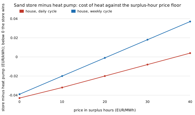
When does a sand heat store beat a heat pump on hourly prices? With 189 GW solar and 137 GW wind and a modelled German price series, a daily or weekly store wins in all 5 years (EUR 0.027/kWh against 0.071); a levy of 0.10/kWh or a surplus-hour price above about 20–35 EUR/MWh removes the win.
What it found
Replaces the flat electricity price of energy-thermal-cost with a modelled hourly price built from real German hourly load, solar and wind (OPSD/ENTSO-E, 2015–2019) and a one-fuel merit order (gas at EUR 54.6/MWh from PyPSA technology-data; surplus hours at a floor of 0, swept to 40). The store buys the cheapest quarter of each cycle; the heat pump pays the November–March mean. With the 189 GW solar and 137 GW wind of the 80%-emissions-cut optimum of energy-mix-sourced, a house-sized sand store cycled daily or weekly beats the pump in all five years (EUR 0.027 and 0.032 against 0.071 per kWh of heat in 2019); monthly and seasonal storage lose. With a fleet like today's there are no surplus hours and the store loses; a levy of EUR 0.10/kWh on both prices makes it lose in every case; a surplus-hour price above about EUR 20–35/MWh ends the advantage. Not from a source: the surplus-hour floor (swept), no storage or grid in the price model, flat winter heat demand, the quarter-cycle charge window. The price is modelled, not a market price, and no taxes or network charges are included in the base case.
A figure from its own output
Paper, code and results
More in Energy supply and dense energy storage
- On real German day-ahead prices, does a sand heat store beat a heat pump, and was the modelled price right?On real German day-ahead prices, does a sand heat store beat a heat pump? Yes at wholesale: daily cycling wins in all 5 years (EUR 0.045–0.062/kWh against 0.070–0.074) and weekly in 4; the earlier merit-order model was flat at EUR 54.6/MWh and wrong; a EUR 0.10/kWh levy removes the win.
- How much is a home battery worth on a time-of-use tariff if it is dispatched optimally?How much is a home battery worth on a time-of-use tariff with optimal dispatch? An LP breaks even at $867/kWh for 10 kWh behind 6 kW PV, against $674 for the best fixed rule ($742 with a 4,000-cycle life); a rolling 36 h plan matches the year optimum (
energy-touwith an optimiser). - How much of an optimal home-battery controller's gain survives a realistic forecast?How much of an optimal home-battery controller's gain survives a realistic forecast? With yesterday's weather or a 7-day mean as the forecast, a rolling LP saves $726 or $691 a year against the fixed rule's $694 (perfect forecast: $892); 84–101% of the gain is lost (
energy-tou-lpwith forecasts). - How much of the home-battery optimiser's forecast loss does re-planning every few hours recover?How much of the home-battery optimiser's forecast loss does re-planning every few hours recover? On PVGIS typical-year data for three US sites, re-planning the LP every 3–12 h instead of daily adds $10–36 a year and closes at most 17 points of the gap to a perfect forecast (10 kWh, assumed tariff);
energy-tou-lp-tmywith receding-horizon re-planning. - Does a clear-sky-index forecast rescue the optimal home-battery controller on real weather?Does a clear-sky-index forecast rescue the optimal home-battery controller on real weather? On PVGIS typical-year data for three US sites, a rolling LP fed yesterday's weather or a clear-sky-index forecast keeps 25–55% of the perfect-forecast gain over the fixed rule at Phoenix and Seattle and none of it at Golden (10 kWh, assumed tariff);
energy-tou-lp-forecaston measured-derived irradiance. - How wrong is the DC approximation of optimal power flow on the IEEE 30-, 39- and 118-bus cases?DC against AC optimal power flow in pandapower on the IEEE 30-, 39- and 118-bus cases: the DC model's cost is 1 to 3 % below the AC optimum (it ignores losses); on the 118-bus case its dispatch is feasible but costs 0.7 to 1.7 % more than the AC optimum once losses are paid, and on the 39-bus case it breaks voltage limits (15 buses at 0.6 of load) at almost no cost difference (modelled benchmark, not a measured system; tightened-limit runs often had no solution). Feeding the AC losses back into the DC model (a loss-adjusted DC) brings the 118-bus cost estimate to within 0.6 to 1.2 % of the AC optimum, but repairs only 13 to 32 % of the dispatch's excess cost and none of case39's voltage violations.
All 39 Energy supply and dense energy storage projects →
Other research topics
Proper scoring & elicitation28Effort & peer prediction9Verification games & slashing19Detection & tolerances14Markets as routers13Prediction-market design9Paying contributors8Decentralised training systems23Digital twins & sim-to-real164LLM chip design loops40Robot manufacturing loops53Ambient AI assistant46Self-replicating manufacturing34Simulation-first design64Engineered clothing45Task-specific AI accelerators40Algorithmic chip-design loops42Open-source purpose-built robots44The software-engineering loop43Adversarial human imitation41Open-source residential construction41Autonomous multi-angle capture34Sensing, imaging and 3D31Energy supply and dense energy storage39Robot societies among people31Agentic co-design of low-cost robots27Laundry-hanging robots25Machine learning on qualitative data23Robots on the building site27Civilizations & group psychology1History & human sciences1
Produced with AI assistance (Claude). Results are from the code in this repository and are simulated or stylised unless the abstract says otherwise; nothing here implies affiliation with or endorsement by any lab, researcher or company cited. MIT licensed.