Can interpretable models predict annual divorce incidence?
research/marriage-divorce-evidence
Original U.S. marriage microdata: interpretable annual-divorce models, schooling/earnings pairings and reproducible held-out validation; no validated personal optimum.
86 tests
What it found
Original ACS, NSFG and NLSY79 microdata analyses separate annual incidence from prevalence. A respondent-held-out enriched additive couple model reduces Poisson loss by about 3.4%; more flexible trees do not improve on it. Includes schooling/earnings pairings, direct contrasts, duration and first-birth checks, trained models and a portable report. A browser app runs the five models on two profiles to give year-by-year divorce odds with explanations, model disagreement and out-of-range flags. Older cohort; observational, not a personal or causal forecast.
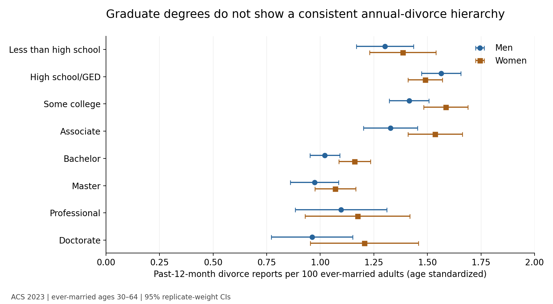
A figure from its own output
marriage-divorce-evidence/figures/annual_degrees.png, written by the project's own experiment code.
Research log
Ongoing: each run adds a batch and an entry, newest first. Source: LOG.md.
2026-10-20 · Flexible models and a pooled nine-survey model: neither beats the single-lens additive models where data are large
Flexible models were tuned with nested, grouped cross-validation on five lenses: LightGBM, boosting, forests, an EBM, an elastic net with pairs, and a stack. None beat the lens's best GLM with a 95% interval above zero. GSS: random forest +0.42 points (−1.55 to 2.25). HCMST: stack +0.65 (−0.11 to 1.43). Tree models fit training folds far better than held-out ones; on GSS, LightGBM scored 44.5% on training folds against 7.4% held out. Shuffled outcomes scored at or below zero for every model. Six large lenses were not run (see NEXT.md).
The pooled Bayesian hazard model covers nine surveys, 321,121 units and 44 inputs, with survey-specific baselines and chained-equation imputation. Held out by person, it beats the single-survey models in HCMST (+4.81 points, 1.88–7.79) and the LA newlyweds (+1.78, 0.60–3.16) and loses in NSFG (−0.85), NLSY79 (−0.50) and Canada (−0.40). Leaving one survey out shows that the effects carry across surveys and the baselines do not. 90% intervals covered 85% of held-out groups. It has not been exported to the app.
[NEXT.md](NEXT.md) lists the action items for later runs: the form inputs, the guided decision flow, the large-lens model runs, the pooled-model export, and the owner asks.
2026-10-20 · Profile report, marital satisfaction by years married, and dating length
New "Profile report" tab in the app (app/report.js, app/report-ui.js): for you and for the person you are looking at, one lens at a time, the 10-year break-up chance with that person, averaged over the partners people like you marry (partner_distribution) and over every partner type of your sex in the survey ("dating everyone"), with model ranges, Dirichlet-resampling intervals on the mix and population percentiles; lowest-risk partner profiles with model disagreement; factor impact (spread across levels) with evidence grades from decision_evidence.json; and the changes with the biggest predicted drop, labelled associations unless graded experimental. Demo couple (woman 36, man 38), NSFG 1995–2023 lens: 5 in 100 with this partner, 6 in 100 (models 3–9) with likely partners, 5 in 100 (3–8) dating everyone; NLSY79 first marriages: 17, 16 and 17 in 100.
reproducibility/satisfaction_by_duration/: GSS 1973–1994 first marriages (13,959): 75% "very happy" at 0–2 years (72–78%), 61% at 16–20 (58–64%), 68% at 41+; unchanged after adjusting for survey year, sex and age at marriage. HCMST 2009→2013 within the same 1,045 couples: −0.14 on a 1–5 rating (−0.19 to −0.09), −0.38 in the first two years. Survivor bias measured: 71% "excellent" among couples who stayed together against 17% among the 102 who broke up by 2015.
reproducibility/dating_length/: HCMST 2009 married couples (118 break-ups): break-up by 2017 8.7%, 8.3%, 8.4% after dating under 1, 1–2, 3+ years; adding dating length to the HCMST lens changes held-out gain by −0.12 points (−0.90 to +0.72) and C by −0.001. Not added as an input; shown with the verified Francis-Tan & Mialon (2015) HRs (0.92, 0.76), which the evidence review already marks not usable in the app.
2026-10-20 · Race detail, family of origin, religion, politics, occupation and wealth: they sort risk but add no held-out skill
Seven lenses refitted with every richer pre-outcome input their data hold, each compared held out with the current model on the same folds (paired person-bootstrap CIs, reproducibility/extended_eval.py, */extended_heldout.csv). No block's gain has a CI above zero in any prospective lens: GSS panels (family of origin, attendance at all 9 levels, prayer, strength, fundamentalism, denomination, religion raised, political views and party, race detail, occupation and prestige, wealth: −1.39 to +0.51 points), NLSY97 (−0.26 to 0.00), NLSY79 (−0.04 to +0.04), NSFG 1995–2023 (−0.05 to 0.00), Statistics Canada family of origin (−0.00) and SIPP couples (occupations +0.11, −0.08 to +0.30; wealth components −0.35). Family of origin as plain yes/no does as well as any finer coding. Canada's religion at the interview "helps" (+0.51) only because it is measured after many separations.
The finer variables do sort risk: Canadian 2017 respondents whose parents never married each other separate at 1.59 times the rate of those raised by both parents, after a parental split 1.30, after a parent's death 1.01; NSFG stepfamilies 1.52, never-married parents 1.20; NLSY79 each sibling 0.96, $100k more pre-wedding wealth 0.90, attending more than weekly 0.83. Every estimate with its CI, source file and row is in the new app/data/predictor_atlas.json (1,159 entries in 18 families, lenses plus verified primary literature; test_predictor_atlas.py traces each to its source).
ACS detail baselines (2019, 2021–24, replicate-weight and age-standardised CIs): one-year divorce per 1,000 by census race group (Asian 8.3, Black 23.6, AIAN 19.5, NHPI 12.1, multiracial 18.9), 18 Asian subgroups (Asian Indian 5.2, Chinese 8.3, Vietnamese 14.4) and 11 Hispanic origins (Mexican 13.7, Puerto Rican 20.3, Dominican 23.1); occupation (detailed, SOC major: healthcare support 25.8 vs architecture and engineering 10.3), industry, household income ($200k+ 6.3 vs under $25k 31.7) and tenure (renters 29.6 vs owners 8.4–9.7), all labelled as measured after any divorce (app/data/acs_occupation_divorce.json).
app/data/race_coverage.json says for every lens which race categories it distinguishes and how each finer form answer maps (NSFG and HCMST: Asian → Other; NLSY: Asian → non-Black non-Hispanic; GSS: Hispanic cannot be placed). Extended models ship in each bundle's models_extended with test vectors (new tests/extended_models.test.mjs, parity to 10<sup>-9</sup>); the app scores none of them until the form asks for the new inputs.
2026-10-20 · Per-couple uncertainty for the "before the wedding" lens
The pre-wedding bundle now carries 50 person-bootstrap refits of its coefficients, with the spline knots and scaling held at the full fit, and engine.cumulativeRisk() returns a point estimate and a 95% interval for the chance a marriage has ended by any horizon. Across 2,000 sampled NSFG first marriages the 10-year interval is 5.2 points wide at the median (9.4 at the 90th percentile).
This is the model's sampling uncertainty only. Transport error between surveys is larger (observed/expected 0.85–1.07 on other U.S. surveys, 0.58 in Canada), and the app should say so next to the interval.
Parity: JavaScript reproduces Python's point estimates and interval ends at 5, 10 and 20 years for 20 test couples to 10<sup>-9</sup>; the bundle grew from 26 KB to 48 KB. ROADMAP B now lists what is done and what remains (intervals for other lenses, a pooled multi-survey model, recalibration to a target population).
2026-10-20 · Before the wedding, from living together: which NLSY97 couples marry, and which split (6,020 first cohabitations)
New pre-marriage lens from the NLSY97 public release (reproducibility/nlsy97_cohabitation_to_marriage/): every respondent's first cohabiting union (born 1980–84, moved in 1994–2023, never married before), followed in the monthly marital and cohabitation arrays. Of 6,020 couples, 2,109 married each other, 3,481 split first and 430 are censored.
Weighted, within 10 years of moving in: 39.1% married the partner and 55.3% split first. With a bachelor's degree or more at move-in, 63.5% married and 29.9% split; with no high-school credential, 21.4% and 74.2%. Moving in before 20: 25.3% married and 72.4% split; at 26–29: 51.9% and 39.1%.
Held out by person (5-fold, yearly Poisson hazards): marrying the partner, additive spline 4.9% deviance gain (folds 4.4–5.7%) against 2.8% for years together alone; splitting first, 9.3% (7.6–10.4%) against 4.7%.
Leakage caught: the partner section's traits (age, schooling, earlier marriage, children) are recorded in a way that depends on how the union ended. Partner schooling is known for couples who split 87% of the time, against 47% where unknown. They are excluded, which cut the split model's apparent gain from 14.9% to 9.3%.
Exported as app/models/nlsy97_cohab_marriage.json and nlsy97_cohab_split.json (stage: before), listed without an adapter. Parity is 300/300 to 10<sup>-9</sup>. ROADMAP A updated: NLSY97 cohabitation done; remaining are Add Health, OSF/Zenodo premarital studies, and PSID / Fragile Families / Understanding Society (403).
2026-10-20 · Browser-trained models: how much your score moves with the training sample
The profile scorer in "Train the models yourself" now shows two things for each model the visitor trained: its estimate on all 29,202 marriages, and the year-10 range across the five fold models from the held-out test. Each fold model learned from a different four-fifths of the women.
For the default profile (the most common answers, wedding in 2020, wife aged 23), the range is narrow for the simple models and wide for the flexible ones: | Model | Full-data estimate | Range across fold models | Width | | --- | --- | --- | --- | | Constant rate | 31.6% | 31.5–31.6% | 0.1 points | | Duration-only GLM | 33.2% | 33.1–33.4% | 0.3 points | | Additive GLM | 21.3% | 18.6–22.9% | 4.3 points | | Depth-4 tree | 34.2% | 26.5–34.6% | 8.1 points | | Boosting | 18.7% | 15.0–23.1% | 8.1 points |
With the wife married at 19, the additive GLM gives 38.3% (33.9–41.7%), the tree 51.0% (41.5–51.2%) and boosting 34.1% (26.1–40.7%).
The tree's full-data estimate sits at the top of its fold range, so its single splits are fragile. A profile's number should be read with a spread of several points even before counting what the survey does not measure.
tests/train_parallel.test.mjs checks that each fold model, after structured cloning, reproduces its fold's held-out predictions to 10<sup>−12</sup>. In headless Chromium at 1200 and 390 px: no console errors, no horizontal scroll.
2026-10-20 · App: per-partner explanations and a default couple at first-wedding ages
Explanations for lenses that score a couple from both partners' sides (the harmonized before-the-wedding lens, NLSY79 couples and individuals) now show one bar set per partner. Each set is exact: its factors multiply (forest: add) to that partner's rate. The page says the couple's rate is the average of the two. The averaged bars they replace were only approximate for the averaged rate. A test checks exactness and the average for every additive model in those three lenses.
The default couple before the wedding is 28 and 30, about the recent U.S. median ages at first marriage, instead of 36 and 38. The married view still opens at 36 and 38, inside NLSY79's data, and a typed age is never changed. On the default lens that couple gets 89% no break-up by year 10. Readable labels were added for the harmonized lens's inputs.
Not done: B's per-couple intervals (#8736) are still a draft, so the tiles show the single model without an interval.
2026-10-20 · App: not engaged yet? Marry each other, or break up first
The before-the-wedding view now answers the earlier question too. For a couple who are dating or living together, workstream A's two HCMST 2009–2017 models (#8662) give the chance of marrying each other within 8.4 years and of breaking up first, chained period by period as the bundles' how_to_combine specifies (app/dating.js). The chain then hands over to the selected pre-wedding lens for the marriage itself.
Two additive models are run: the full one, and the harmonized one A checked on HCMST's 2017 cohort (#8727; AUC 0.79 for marrying and 0.85 for breaking up by 2022). The page shows their range.
A couple living together for 3 years (27 and 29, bachelor's degrees, parents approve, rating the relationship excellent and good): 60.4% marry each other within 8.4 years (models 50.9–70.0), 31.7% break up first (21.9–41.6), and 7.9% are still together and unmarried. The same couple rating it fair and living apart: 9.2% marry (6.5–11.9) and 86.9% break up first (81.9–91.9). Across all 939 couples, 21.9% married and 54.0% broke up first.
The two outcomes were modelled separately, so the split is approximate, and the page says so.
The hand-over multiplies two estimates from different surveys (marrying within 8.4 years, times no break-up in the first 10 years of marriage) and is labelled as an approximation.
2026-10-20 · In-browser training runs the five folds in parallel: 45.5 s → 18.8 s
The "Train the models yourself" panel now runs a pool of workers, by default one per spare core: at most five, and fewer on devices reporting 4 GB of memory or less. Visitors can choose 1–5 threads.
Each worker loads the NSFG extract once and takes tasks from a shared queue: the five held-out folds, then the refits on all marriages. When the last fold arrives, the next free worker merges the folds and computes the metrics. Arrays move between threads by transfer, not copy, and the page's own thread only routes messages.
All five models at the Python settings, in headless Chromium on a 4-core cloud machine: | Threads | Wall time | Longest main-thread stall | | --- | --- | --- | | 1 | 45.5 s | 93 ms | | 3 (the default here) | 18.8 s | 57 ms | | 4 | 17.6 s | 62 ms | | 5 | 17.5 s | 86 ms | A 390 px run with 25 boosting rounds on 3 threads took 6.9 s.
The metrics are identical at every thread count: GLM 5.688%, tree 3.333%, boosting 6.30%, C 0.695 / 0.651 / 0.703. Merging folds in the page took stalls to 177 ms at 5 threads, so the merge moved into a worker.
Cancel stops every worker. There were no console errors and no horizontal scroll. tests/train_parallel.test.mjs computes the folds in scrambled order through structured cloning and matches the single-thread result to 10<sup>−12</sup>. No real phone has been timed yet.
2026-10-20 · Train the models yourself: the NSFG 1995–2023 lens retrained in the browser, matching scikit-learn
The app has a new "Train the models yourself" panel. A background worker downloads a 374 KB public extract of the NSFG 1995–2023 women's first marriages: 29,202 marriages, 10,529 dissolutions and 249,868 marriage-years. It contains only inputs fixed at or before the wedding. The worker then refits the lens in plain JavaScript with the Python pipeline's person-held-out five folds.
The NSFG files are U.S. government works and not under copyright, so the extract can be published. The NCHS data-use terms are recorded in the file: statistical use only, no attempt to identify anyone, no linkage.
Held out, the browser reproduces scikit-learn 1.7.2 on the same extract: | Model | Browser | scikit-learn | | --- | --- | --- | | Duration-only GLM | 0.645% | 0.645% | | Additive spline Poisson GLM | 5.688%, C 0.6947 | 5.688%, C 0.6947 | | Depth-4 Poisson tree | 3.333%, C 0.6512 | 3.333%, C 0.6512 | | Poisson gradient boosting (250 rounds) | 6.298%, C 0.7029 | 6.297%, C 0.7028 | scikit-learn on the extract also matches the shipped lens's 5.688% and 6.289%, which confirms the extract.
The JS GLM's coefficients equal scikit-learn's within 4×10<sup>−14</sup>. It uses Newton's method with the Hessian accumulated per person and per marriage year, so a fit takes 0.7 s. Gradient boosting fits histogram trees with per-person runs and child-histogram subtraction, at about 21 ms per round.
A full run took 35 s in Node and 44 s in headless Chromium at 1200 px. At 390 px with 25 boosting rounds it took 13 s, but boosting's gain fell to 3.85%. The main thread never stalled more than 68 ms, cancelling works, there were no console errors and no horizontal scroll. No real phone has been timed yet.
After training, the models are refitted on every marriage, and a visitor can score a profile with the models they just trained. tests/train.test.mjs checks the coefficients to 10<sup>−6</sup>, the held-out gains (0.001 points; 0.15 for boosting), the C indices, O/E and the extract's sample.
2026-10-20 · Before the wedding, checked on a later cohort: 2009 dating models predict 2017 couples
The two HCMST before-the-wedding models (marry the partner, or break up first) were trained on couples unmarried in 2009. They were scored, without refitting, on the 777 couples unmarried in HCMST's fresh 2017 sample, using a harmonized variant without parents' view or religion (not asked in 2017).
By 2020: marrying AUC 0.767 (16.5% observed, 15.8% predicted); breaking up first AUC 0.838 (33.1% vs 34.4%). By 2022: marrying AUC 0.786 (21.7% vs 21.6%); breaking up first AUC 0.847 (43.8% vs 44.9%). That is at least as good as the 2009 held-out AUCs (0.72 and 0.70). This is one later cohort of the same survey, not a different population.
Data fix: 8 weddings to the 2017 partner newly reported in 2022 show up only in w3_when_married_yr plus w3_partner_source, because the derived w3_partner_type was not updated. Counting them raises 2022 marriages from 65 to 73.
The bundles now carry the harmonized model, the external results and stage: before (the convention in couple.js, #8713). Parity is 320/320 to 10<sup>-9</sup>. ROADMAP A item 3 is done.
2026-10-20 · App: the harmonized before-the-wedding model is the default lens
Workstream B's harmonized model (#8684) now scores couples in the app, and it is what "Before the wedding" opens on. It uses only facts knowable on the wedding day (NSFG 1995–2023, 43,336 first marriages; held-out C 0.661). Each partner is scored as the surveyed spouse, and the two rates are averaged. Unanswered inputs take the survey's most common answer, and the page names them.
A typical engaged couple (28 and 30, bachelor's degrees, living together first, no children before) gets 7.4% break-up risk by 5 years, 12.5% by 10 and 19.1% by 20. That is the 2nd percentile among NSFG's first marriages, whose median 10-year risk is 28%. A younger couple (22 and 23, a child before the wedding, not living together first) gets 22.5% by 10 years (32nd percentile). It is a single model, so the page shows no model range; the other pre-wedding lenses give the spread.
Next: chain the HCMST dating-couple models (marry vs break up first) into this lens for couples not yet engaged.
2026-10-20 · App: "Before the wedding" is now the calculator's default question
The owner's refocus: predict divorce before marrying, for a couple or a candidate partner. The calculator now opens on Before the wedding. Its lens list, summary, just-me and candidate views use only the eight lens views whose clock starts at the wedding and whose inputs are known by then (NSFG 1995–2023 and its both-sexes view, NLSY97, NLSY79 first marriages, SIPP first marriages, Statistics Canada, NSFG 2002 and its model family). The projection starts on the wedding day, and question groups only married-couple lenses read are hidden. The nine married-couple and non-divorce lenses sit behind Already married, unchanged.
For a typical engaged couple (28 and 30, bachelor's degrees, living together first, no earlier marriages or children, U.S. Midwest), 10-year break-up risk is 6.7% in NSFG 1995–2023 (models 3.8–9.7), 7.8% in NLSY97, 16.5% in NLSY79, 17.4% in SIPP, and 24.7% and 20.6% in the two NSFG 2002 lenses. Statistics Canada abstains (no Canadian region). Cohorts and outcomes differ, so the levels are shown side by side, never pooled. Ranking skill from pre-wedding facts is modest: C 0.63–0.66 within surveys in the leakage-free models.
Next (ROADMAP C): B's harmonized pre-wedding lens as the default once #8684 merges, and the HCMST dating-couple chain for couples not yet engaged.
2026-10-20 · "Before the wedding" lens exported to the app
New bundle app/models/prewedding_harmonized.json (26 KB): the harmonized pre-wedding additive model fitted on 43,336 NSFG 1995–2023 first marriages, inputs from either partner's point of view and nothing measured after the wedding. Held out by person in NSFG: C 0.661, AUC at 10 years 0.656, observed/expected 1.03. Applied unchanged elsewhere: NLSY97 C 0.647 (observed/expected 0.99), NLSY79 0.621 (1.07), SIPP 0.626 (0.85), Canada 0.611 (0.58).
Cross-fitted population reference: median predicted 10-year dissolution 28% (10th–90th percentile 16–51%); out-of-distribution percentile among held-out marriages.
engine.js gains constant spline extrapolation (wedding year held at the edge, not extrapolated) and mode imputation of Unknown answers for models and the OOD score; tests/prewedding.test.mjs matches 60 of 60 Python predictions and distances. The lens needs workstream C's form adapter to become the default.
2026-10-20 · Before the wedding: leakage audit, harmonized features and cross-dataset validation on five surveys
Question: how well can divorce be predicted from facts known on the wedding day? Built one harmonized pre-wedding table per first-marriage lens (NSFG 1995–2023 43,336 marriages; NLSY79 6,768; NLSY97 5,076; SIPP 176,303; Canada GSS 48,656), each reproducing its lens's published sample exactly, with strict timing rules (reproducibility/prewedding/SPEC.md).
Leakage audit: four lenses used information from after the wedding. NLSY79 spouse traits from the first post-wedding interview (published 5.07% → 4.52% additive, 5.60% → 4.54% boosting), NLSY97 spouse education and pregnancy defined by a later birth (4.82% → 4.50%), NSFG degrees earned in the wedding year (4.74% → 4.52%), Canada region at interview (3.18% → 3.07%); SIPP's main model was clean. Missingness itself leaks (in NLSY79 29.7% of marriages with a blank roster spouse ended within two years against 6.1%), so the harmonized models use no missing indicators or "Unknown" levels.
Within each survey, held out by person: C 0.634–0.664 and AUC at 10 years 0.66–0.68 for the best model, 10-year observed/expected 0.99–1.03. Boosting beats the additive model by at most 0.7 points and not at all in NLSY97; a discrete-time logistic hazard equals the additive Poisson model.
Across surveys (20 train→test pairs): ranking transports within the U.S. (C 0.61–0.66; NSFG → NLSY97 0.647 with observed/expected 0.99) but levels are off by up to a third, and U.S. models predict 1.5–2.2 times Canada's divorce while ranking at C 0.59–0.61. Wedding year must not be extrapolated: NLSY97's additive model loses 31–38% on older cohorts unless it is dropped. NSFG transports best, so it is the candidate for a "before the wedding" app lens (next round).
2026-10-20 · Decision evidence: what changing a decision did in trials, and how strong the evidence is for each input
New reproducibility/decision_evidence/: 46 records. 35 are evidence about decisions (12 randomised trials or trial subgroups, 7 meta-analyses of trials, 6 quasi-experiments, 1 selection model, 7 adjusted observational including 5 from this project, 1 cross-sectional, 1 review) and 11 are decision-aid standards and risk-communication studies. Each has design, population, n, outcome, effect, follow-up, caveats, verbatim quote and DOI. All 46 pass the literature-evidence checks (quote fragments verbatim in the cached source, every quoted number present, every stored value printed or recomputed from printed inputs) and all 36 DOIs match Crossref. Provenance: 19 full text, 21 abstract only, 1 secondhand, 5 from this project's own METHODS files. Source texts stay out of Git.
Relationship education: Army PREP lowered divorce at 2 years (7.6% vs 11.9%; 8.1% vs 14.9% at the higher-risk site, none at the other); an engaged/newlywed trial found 11% vs 24% dissolution at 3 years, but a one-session film-discussion arm matched 15 hours of skills training. The federal trials are null on stability: Building Strong Families 57.4% vs 60.5% still together at 3 years (p = .053, wrong direction), Supporting Healthy Marriage 81.5% vs 81.5% at 30 months (impact 0.0, SE 1.0); ACF-funded programmes pooled show small quality gains (d = .114) and no stability effect.
Couple therapy improves satisfaction (d = .585 vs no treatment over 30 RCTs) but no trial compares divorce with untreated couples over years; 25.7% and 27.9% of seriously distressed couples had separated 5 years after IBCT or TBCT.
Causes: no-fault divorce laws brought divorces forward (+0.27 per 1,000 people a year in the first two years) without a lasting rise; plant-closure job loss raised divorce 18% in Sweden (CI includes 1) and not detectably in the US; $25-50k lottery wins changed nothing; a welfare work-incentive trial cut divorce 3.5 points among recipient families but not applicants. No experiment or instrument estimates age at marriage, education, cohabitation or religious attendance effects on divorce.
FACTORS.md / factor_grades.json grade all 10 changeable inputs (numbers copied from verified records; the build fails if a grade claims more than its evidence). DESIGN.md is a 14-item IPDAS and risk-communication checklist mapped to the app's views with today's status (absolute risks with time frames: met; icon arrays, evidence grades beside what-ifs, interventions as options, user testing: not yet). app/data/decision_evidence.json is the app-ready export; DecisionEvidenceTests re-check it.
2026-10-20 · Before the wedding: which unmarried couples marry, and which break up first (HCMST 2009–2017)
New direction from the owner: predict divorce before marrying. Every lens so far starts at the wedding. This one starts earlier: the 1,081 HCMST couples who were together but not married in early 2009 (dating or living together, 378 of them same-sex), followed to 2017. Of the 939 re-interviewed, 160 married each other and 400 broke up first. Only 9 of the 160 marriages had ended by the last report, far too few to estimate whether they last, so the app should hand over to a marriage lens (NSFG and others) after the wedding (reproducibility/hcmst_dating_to_marriage/).
Weighted, by about 8.4 years: 21.9% married and 54.0% broke up first. Couples who called their relationship "excellent" in 2009 married 37.0% of the time (broke up first 40.3%); "fair", 4.1% (79.3%). Cohabiting couples married 34.0% of the time against 14.3% for couples living apart. Couples whose parents approved married 31.6% of the time against 11.3% where parents were neutral or unsure.
Held out by couple (5-fold), two cause-specific per-period logistic models on 2009 answers: marriage AUC 0.726 (log-loss gain 7.9%, folds 1.4–20.5% with only 160 weddings); break-up before marrying AUC 0.706 (9.3%, folds 5.9–12.8%). The depth-2 trees and the period-only baselines add almost nothing.
Exported as app/models/hcmst_dating_marriage.json and hcmst_dating_breakup.json with how_to_combine (still-dating survival times each period's marriage share). Listed without an adapter; parity 240/240 to 10<sup>-9</sup> (app/tests/hcmst_dating.test.mjs). The Stanford repository record gives HCMST's licence as ODC PDDL 1.0.
2026-10-20 · Compare many scenarios in the calculator, lens by lens
The owner asked for the app to "easily compare many scenarios". A new "Compare options" tab (framed as a decision aid: each saved scenario is an "option", the baseline is "your current plan") saves the full form (both profiles, the marriage, every optional lens question and the published-evidence answers) as named scenarios, up to 50, with rename, duplicate, delete, reorder, load-into-the-form-and-re-save, and "vary one thing": copies that differ in one answer across its allowed values (age at the wedding, years married, living together first, degree, schooling, relationship quality, marriage happiness, religious attendance, work hours, wages, earlier marriages and children, family of origin, relationship status, how you met, a baby expected, home ownership), at most 12 per click, labelled by the change.
The comparison is one column per lens at a horizon the lens supports (defaults: the three lenses summary.js ranks most relevant to the baseline). Each cell gives the expected break-ups out of 100 couples like you (and the percentage) at one horizon shared by every option, with the range across the lens's models; the change from the current plan in points, with the smallest-to-largest change across the models, and as a ratio; and a paired verdict from each scoring model's own difference: "models agree" (every model moves the same way, each by at least 1 point), "most models agree (k of n)" (a strict majority, median move at least 1 point), or "cannot tell apart" with the reason (the models disagree on the direction, or the change is under 1 point). Overlapping min–max ranges are not used for this: they measure how much the models disagree on the level, not on the difference. Where a lens publishes posterior draws (none does yet), the share of draws in which the option is lower is reported too; the population percentile, and flags for steps outside the lens's data or a couple more unusual than 90% of its people; a lens that refuses shows its reason. A small chart per lens draws each scenario's model range and average against the baseline. Nothing is pooled across lenses: the CSV has one row per scenario × lens × horizon, and the numbers are summariseLens's own (the form-to-inputs mapping moved from app.js to scenarios.js so saved scenarios and the live form share it).
Example from the browser check: three scenarios that differ only in both partners' relationship quality (Excellent, Good/Fair/Poor for one partner) move HCMST's 8.4-year break-up chance from 16.1% to 20.1%, 25.0% and 30.9% (+4.0, +8.9, +14.8 points on average). The worst reads "Most models agree (2 of 3): higher risk by 21.0–23.3 points; 1 does not move" (the third model does not use relationship quality). NLSY79 couples and the Los Angeles newlyweds, which do not read that answer, show "No difference: none of the 5 models move".
Privacy: hostility, abuse, substance use, low mood and childhood-adversity answers, and the published-evidence answers on destructive conflict (both partners), depression, alcohol problems and neuroticism (both partners), never go into a share link (this also changes the single-scenario link, which used to carry the published-evidence answers), the CSV or this browser's storage; they reach an exported JSON file only when the user ticks "include sensitive answers". Links use the single-scenario link's whitelist, with later scenarios stored as changes from the first (six scenarios: 2.4k characters). Imports reject any unknown key, field or value and import nothing; the 50-scenario cap applies to saving, varying, links and files, with a message.
Tests: tests/scenarios.test.mjs (12 tests; 109 Node tests pass in all). Headless Chromium at 1200 and 390 px, light and dark: no console errors, no page-level horizontal scroll (the grid scrolls inside its own box), every input labelled, arrow keys reach the tab, scenarios survive a reload and a share link, and the page works with storage blocked.
2026-10-20 · Every lens scored in the app: relationship quality, marriage happiness, newlyweds, Census and Canada, with a summary that pools nothing
The calculator now scores all 15 lenses (13 bundles plus the NSFG 1995–2023 both-sexes view); only Fair's affairs surveys stay listed, as their outcome is not divorce. New form adapters (app/lens-adapters.js) map the form onto each bundle's documented inputs: HCMST (relationship quality, married or not, same-sex, how you met, years together, party pair), GSS panels (marriage happiness), NLSY79 and NLSY97 first marriages (with the spouse's traits), NSFG 1995–2023 (wife's report, and each spouse's own report), Statistics Canada (one partner at a time, 2017 cycle), the Los Angeles newlyweds (satisfaction, self-reported hostility, conflict questions mapped to observer-code percentiles and labelled an unvalidated approximation), SIPP first marriages, SIPP couples one year ahead (both spouses' earnings, net worth, debt, home ownership) and ACS one-year incidence (labelled cross-sectional).
Honesty rules in code: an input the model has no "unknown" level for, left blank, means no number from that lens and names the question; documented imputations (training medians, "Unknown" levels, the NLSY79 "not tested" flags) are used and listed. Each lens shows only the horizons its follow-up covers (GSS 2 years; HCMST 2.2/4.1/8.4; newlyweds 2.3–12; SIPP couples and ACS 1 year): periods combine as each bundle's how_to_combine says and nothing is extrapolated or given a lifelong figure.
Out-of-distribution checks now run per lens on that lens's own rows (the old check built NSFG rows for every bundle); inputs a person did not give are neutral in the distance. The NLSY79 couples bundle gains its OOD spec and an annual-rate population reference from app/tools/nlsy79_reference.py (re-derived from the public release; held-out gains within 0.0028 points of the committed ones; the bundle's prefix is byte-identical, and the parity test now runs: 50 of 50 distances to 1e-9).
population.js converts every published reference shape (standard p1–p99, cells lists whose p5/p10 keys are horizons, GSS horizon_N blocks, HCMST per-model cells with suppressed percentiles, the NLSY79 annual-rate cells) into one form, compares the couple on the reference's own model and quantity, and refuses unknown shapes. The GSS 4-year block is not used because its model is not exported.
A "Summary across lenses" panel lists every lens's estimate, model range, percentile, held-out skill and data fit, then says where the lenses agree on relative risk, which disagree internally, and which is most relevant (in its data, typical of its people on the inputs given, skilful held out). Just me, candidates, the dashboard (non-negotiables, what-ifs) and batch CSV (new optional columns, results at each lens's own horizons) work through every lens that has the blocks they need, and say so where a lens lacks one. ACS subgroup baselines (12,760 cells) show next to the population comparison.
Tests: 96 Node tests pass (new adapters.test.mjs, summary.test.mjs), including every model input filled with a level the model knows, period-product parity, refusals, horizons, per-lens OOD and every reference conversion. Headless Chromium at 1200 and 390 px, light and dark: no console errors, no horizontal scroll, every input labelled.
2026-10-20 · SIPP and ACS: 176,303 first marriages, the only wealth data, and divorce baselines for 12,760 subgroups
SIPP retrospective first marriages (Census; 2001, 2004, 2008 marital-history modules and the 2021 and 2025 annual files, non-overlapping): 176,303 first marriages from 1960 in 102,497 households, 60,868 dissolutions dated by separation year, 8,331 widowhoods censored. Module record counts and weight totals match Census documentation. Held out by household: gradient boosting 4.82% (4.69–4.97%), additive spline 4.07%, C 0.65; education dated by the wedding (2001–08 modules) adds +0.28 points (0.24–0.32). Spouse traits are excluded because the files describe only the current spouse. 74.0% of first marriages are still intact at 10 years; the five surveys agree within 4.5 points.
SIPP prospective couples: spouses linked within households and followed one year with Census longitudinal weights, seven year-pairs 2018→19 to 2024→25: 33,698 couple-years, 17,960 couples, 312 separations or divorces. Both spouses' demographics and education: 5.77% (3.66–7.86%), AUC 0.695. Adding earnings, income, net worth, debt, home ownership and employment changes held-out gain by −0.79 points (−2.82 to +0.91) and AUC by +0.000. Alone, the gradients are steep (negative net worth 24.4 per 1,000 a year against 4.9 at $1M+; renters 19.5 against owners 8.9).
ACS 2008–2024 (17 years, 53.6M person records): one-year divorce incidence fell from 19.3 per 1,000 married people in 2008 to 13.2 in 2024; pooled 2019 and 2021–24, 13.6 (13.5–13.7) from 7,569,524 people and 89,289 divorces. app/data/acs_divorce_baselines.json holds 12,760 subgroup cells (one- and two-way crosses, and state × age × education × duration × times married) with replicate-weight CIs, each with at least 200 people. "Unknown duration" cells are dropped: they are exactly people who divorced and remarried within the year. Held out by household (cross-sectional; inputs measured after any divorce): boosting on background inputs 3.94%, AUC 0.68; adding income, employment and occupation 4.91%, AUC 0.70.
All three bundles carry a population_reference in the standard shape. Engine notes: quantile spline knots that repeat at piled-up values break JS/sklearn parity, so the couple model uses evenly spaced knots. Listed in the app; scoring needs form adapters.
2026-10-20 · NSFG 1995–2023: every survey cycle pooled, held-out skill more than doubled
New data: all eight NSFG female cycles (1995–2023) and all seven male cycles from 2002, official CDC files. Every file's record count matches the official sample size and weighted totals match NCHS's published populations; 2017–19 dissolution counts match the codebook exactly; the 2002 women reproduce the existing lens exactly (4,126 marriages, 1,492 dissolutions). 29,202 women's first marriages and 10,529 dissolutions (both sexes: 43,336 and 15,256).
Timing and leakage: months suppressed after 2015 are imputed within the published years (mean error +0.3 months on exact-date cycles; skill unchanged on exact-date cycles alone); the wife's degree counts only when dated on or before the wedding; anything measured at interview (education, current religion, income, residence, husband's education) is excluded.
Held out by person (95% person-bootstrap CIs): gradient boosting 6.29% (5.85–6.73%), C 0.703, AUC 0.72 at 5 and 10 years, top tenth 13.5 times the bottom; additive spline GLM 5.69%, C 0.695. The 2002 lens refit on the same folds: 2.86%, C 0.645. On the 2002 women alone boosting still adds +1.29 points. Out of time (trained on pre-2000 weddings, tested on 12,460 weddings 2000–2023): boosting 6.73%, C 0.713, observed/expected 0.99; the 2002 lens 4.41% with observed/expected 0.84.
Rate ratios (additive GLM, cluster bootstrap): wife married at 17 against 23, 2.63; at 28, 0.60; bachelor's degree by the wedding 0.63; husband's prior children 1.35; husband married before 1.26; different race-ethnicity 1.29; not raised by both parents 1.30; no premarital sex against 4.8 years 0.68; born outside the U.S. 0.85; weddings in 2020 against 2000, 0.82. Living together first: 1.01 (0.97–1.06). Survival: 79.4% intact at 5 years, 66.7% at 10, 51.8% at 20.
The bundle carries the GLM and boosting as scoring models, a both-sexes model, an out-of-distribution score, a population_reference in the standard shape (median predicted dissolution 17.8% / 30.2% / 46.1% at 5 / 10 / 20 years) and partner distributions. Parity 4/4 to 10<sup>-9</sup>. Listed in the app; scoring needs a form adapter.
2026-10-20 · Los Angeles newlyweds: trained-observer conflict codes add nothing to divorce prediction
New data: Smith, Block & Karney's public OSF release (hxn84) of 368 low-income, mostly Hispanic Los Angeles newlywed couples followed for about 12 years, 145 divorced. Both spouses are measured, and couples' conflict discussions were coded by trained observers (IFIRS positivity, negativity, effective communication). Hostility, described elsewhere as observed, is a 14-item self-report questionnaire, so it is a separate block here.
Reproduction: 368 couples and 145 divorces exactly; all 22 Table S1 means and SDs and all 8 Table S8 percentages within rounding; Table S11 baseline hazards match as Bayesian posterior means; Table S12 survival odds ratios match approximately (same signs; wife vulnerability the only predictor whose CI excludes 1, as published). Table S2.1's "Included" and "Excluded" headers appear swapped in the supplement.
Held out by couple (20 × 5-fold, nested tuning, 1,000 couple resamples): the best model (ridge on all inputs) gains 3.42% (1.47–5.30%) in log loss over an interval-only model, C-index 0.63 (0.58–0.67), AUC 0.67 by 12 years, Brier 0.218 against 0.239. Observed codes alone: 0.63% (−0.07 to 1.26%), C-index 0.53.
The Gottman-style test: adding the observed codes to satisfaction, socioeconomic risk and each spouse's vulnerabilities changes held-out gain by −0.05 points (−0.51 to +0.39) and the C-index by +0.004 (−0.010 to +0.018). Socioeconomic risk and vulnerabilities over satisfaction add +1.32 points (+0.14 to +2.70). Per SD: husband satisfaction 0.78, wife satisfaction 0.72, self-reported hostility 1.33 (husband) and 1.38 (wife); of the observed codes only the wife's effective communication excludes 1 (0.81), and not after adjusting for satisfaction and hostility.
The bundle lists each observed code with a self-report question for app users and says plainly that the model was trained on observer codes, so self-ratings are an unvalidated approximation. Population reference in the standard shape (median 12-year divorce risk 0.38). Test vectors are synthetic. Limits: one low-income Los Angeles sample with no external validation; 36 divorces were first reported after a missed follow-up; the null covers these three codes, not Gottman's own coding or physiological measures.
2026-10-20 · NLSY97 first-marriage lens: the young cohort, marriages through 2024
Official NLSY97 public release (BLS, no login; sha256 recorded), streamed out of the 8 GB CSV without unzipping. Counts match the codebook: 8,984 respondents, round-1 weights summing to 19.38 million, 5,252 ever married, first-marriage ends 1,820 divorced, 20 widowed, 45 unknown.
5,076 first marriages (62 same-sex marriages excluded; 10 undatable dropped), 1,906 dissolutions (first month marked separated or divorced), 42 widowed and censored, 50,592 person-years. Predictors are fixed at or before the wedding; partner traits come from the household roster at the first interview after it (median 7 months), because the partner section only describes partners who are no longer current, which would leak the outcome.
Held out by person (5 folds × 3 repeats; 400 person bootstraps): gradient boosting 4.91% (4.23–5.52%), C 0.677, AUC 0.697 at 5 years and 0.686 at 10; additive spline 4.68%, C 0.672. Top decile 9.5% a year against 0.94% in the bottom; observed/expected 0.96. Weighted survival: 81.6% intact at 5 years, 67.7% at 10, 52.0% at 20.
Ablation: dropping partner traits loses 0.32 points (0.14–0.50), relationship history 0.23, both 0.68; every other block about 0 given the rest. Rate ratios (additive, adjusted associations): age at marriage 34 against 20, 0.55; spouse 16+ years of school against 12, 0.64; four years of living together first, 0.68; 2+ earlier live-in partners 1.33; lived with neither parent at 12 against both, 1.45; better mental health (MHI-5 87 against 53), 0.72.
The bundle carries an out-of-distribution score, a population_reference in the shape population.js reads (median predicted dissolution 17% / 30% / 47% at 5 / 10 / 20 years) and a partner distribution. Parity 3/3 on 80 rows. Listed in the app; scoring needs a form adapter.
2026-10-20 · Statistics Canada GSS Families: 48,656 first marriages from four survey cycles
New data: Statistics Canada's General Social Survey on Families public-use files (1995, 2006, 2011, 2017; Open Licence; CSVs from Borealis, whose MD5s match). All 53 documented figures compared (record counts, weight totals, end-type and marital-status frequencies) match the files.
48,656 first marriages (weddings 1950–2016) and 14,235 dissolutions (separation, or divorce without a recorded separation); 3,875 widowhoods censored; 878,794 person-years over the first 30 years. The 2011 cycle has no age at the spouse's death, so its 1,283 widowed marriages are censored at times drawn from 2006/2017 widows of the same sex and wedding decade instead of being dropped.
Held out by person (5 folds, person-bootstrap CIs): gradient boosting 3.57% (3.32–3.82%) over a constant rate, Harrell's C 0.656, AUC 0.685/0.691/0.690 at 5/10/20 years, top tenth against bottom tenth 6.9 times the rate; additive spline 3.18%. Out of time (trained on pre-1990 weddings, tested on 15,488 later ones), boosting keeps 3.37% with observed/expected 1.03; the additive model over-predicts later weddings (0.82).
Rate ratios (design bootstrap): lived together first 1.81 (1.70–1.92), child before the wedding 1.54, married under 20 1.49 against 20–24, 35 or older 0.60, not with both parents to 15 1.30; an earlier common-law union with someone else, birthplace and the respondent's sex show no clear effect. Weekly attendance at interview 0.48 is a labelled sensitivity (measured after the fact).
Survival: 85.4% of first marriages intact at 10 years, 76.1% at 20; 75.3% and 62.5% for those who lived together first. Canadian women's 10-year survival exceeds NSFG 2002's by 10–23 points in every comparable cell; the surveys differ, so the comparison is descriptive. Common-law unions are described separately: 57.7% together at 10 years, 43.7% later married.
Left out of the shipped models because they would leak the outcome or postdate it: education and religion (measured at interview), the partner age gap (missing for 7–19% of ended marriages against under 2% of intact ones), the survey's union-rank variable. bundle_export.py now exports gradient-boosted and random-forest Poisson models in the engine's existing formats and refuses estimators it cannot reproduce. Parity: 3/3. Listed in the app; scoring needs a form adapter.
2026-10-20 · NLSY79 rebuilt from the public release, a from-the-wedding NLSY79 lens, and the GSS marriage-happiness panels
NLSY79 full public release (BLS, no login). Re-running the four ml_couples scripts unchanged recovers the published sample exactly (40,818 intervals, 5,735 people, 726 divorces, the same folds). Held-out gains match within 0.003 points (additive enriched 3.4016% committed, 3.3988% rebuilt): numpy's sort orders tied incomes differently on this CPU, moving 59 intervals across a wage quartile. app/tools/nlsy79_reference.py can now add an out-of-distribution score and a population reference to the couples bundle; they are not attached yet, because the app's typicality check builds NSFG-shaped rows and needs an NLSY79 row first.
New lens: NLSY79 first marriages from the wedding, 1981–2022. 6,645 marriages, 2,727 legal divorces, 110,538 person-years; predictors from the last interview before the wedding, spouse traits from the first one after, with delayed entry so a missing spouse cannot leak an early divorce. Held out by person (5 folds × 3 repeats, 500 person bootstraps): gradient boosting 5.6% (5.1–6.4%), additive spline 5.1% (4.4–5.8%), Harrell's C 0.656, AUC at 5/10/20 years 0.70/0.69/0.68. The top predicted tenth divorces by year 10 at 53.9% against 26.0% overall. Ablation: spouse traits add 0.54 points, age at marriage and wedding year 0.40, delinquency 0.19; schooling, AFQT, race, sex and income about zero.
New lens: GSS panels 2006–2020 (official NORC files; every panel size matches NORC's documentation). 4,453 two-year follow-ups of married people, 203 divorces or separations. Two-year dissolution by self-rated marriage happiness: very happy 2.5% (1.9–3.2%), pretty happy 5.5% (4.2–7.0%), not too happy 23.6% (16.5–31.2%). Re-interview barely depends on happiness (74.7%, 77.2%, 73.5%), and re-weighting for it changes the rates by under a point. Held out (5 folds × 10 repeats): happiness alone 5.6% log-loss gain, AUC 0.629; additive logistic 8.6% (4.8–12.3%), AUC 0.727. Odds ratios: not too happy 10.9 against very happy, divorced before 2.51, 0.64 per 10 years of age. Cross-sectional GSS 1972–2024 (57,753 ever-married people, supporting only): marrying before 20 has adjusted odds 2.52 of ever divorcing against marrying at 23–25.
population.js now reads only the standard reference shape, so the new bundles' differently shaped summaries (per-cell lists, annual rates, 2-year horizons) show "no reference" until they are converted, instead of a percentile read off the wrong quantity. Both lenses are listed in the app; scoring them needs form adapters, next.
2026-10-20 · HCMST couples lens: relationship quality, unmarried and same-sex couples, checked on a later cohort
New data: Stanford's How Couples Meet and Stay Together, official files from data.stanford.edu. The 2009 cohort gives 3,009 partnered couples (1,928 married, 1,081 unmarried, 474 same-sex), re-interviewed through 2017: 8,046 couple-periods and 527 break-ups, exactly HCMST's own combined break-up variable (503) plus the 24 wave-6 break-ups. Every sample count matches Stanford's documentation. 98 partner deaths are censored.
Logistic per-period hazards held out by couple (5 repeats × 5 folds, 1,000 couple-bootstrap CIs). The additive core model gains 25.5% (22.6–28.3%) in log-loss over a period-only model, C-index 0.878 (0.864–0.892), calibration slope 0.98; the riskiest tenth breaks up at 4.3 times the average rate. Relationship quality alone gains 6.2%; boosting (26.3%) adds little and is not exported. Within married couples the C-index is 0.84 (0.80–0.88), unmarried 0.755, same-sex 0.83.
External check: the core model trained on 2009 and applied to the separate 2017 cohort gives AUC 0.925 (0.906–0.941) for break-up by 2020 (observed/expected 0.90) and 0.928 by 2022 (1.03).
Break-up by 2017 by rated relationship quality: excellent 14.3%, good 36.3%, fair 55.0%, poor or very poor 60.3% (62 couples). Married couples: 4.6%, 18.9%, 27.5% and 47.1%. Odds ratios per period, holding the other inputs fixed (associations): good 2.57, fair 5.11, poor 13.7 (7.1–29.5) against excellent; not living together 3.56; unmarried 2.08; each doubling of years together 0.66; two women against a man and a woman 2.57. Meeting online (0.89, 0.61–1.18), interracial pairing, mixed party, different religions and parental disapproval show no clear effect.
The bundle carries a population_reference (weighted p1–p99 of held-out predicted break-up by 2.2, 4.1 and 8.4 years, by marital status, quality, age, education, how met, interracial and duration; cells of 100+ couples, extreme quantiles only for 200+/500+). Median 8-year break-up: 11.2% overall, 7.1% married, 60% unmarried. All five exported models match Python to 10<sup>-9</sup> (app/tests/hcmst.test.mjs).
Limits: one partner reports for both; attrition is heavy (46% response by wave 5), assumed unrelated to break-up given the inputs; the penalty was chosen once on all couples, a slight optimism; the 2017–2020 window includes the pandemic's start. The lens is listed in the app; scoring it needs a relationship-quality field on the form, next.
2026-10-20 · Published evidence, re-verified, in the app: what the surveys don't measure, Gottman's base rates and CDC/NCHS baselines
New reproducibility/literature_evidence/: 286 records of published evidence on divorce predictors, each with a verbatim quote and a DOI. Provenance: 249 checked against the full primary text, 31 against an abstract only, 6 secondhand (Gottman Institute FAQ, press release, transcription). All 286 pass scripts/verify_quotes.py against their cached sources; without the cache it still recomputes every derivation.
The mechanical re-check changed 108 of the 286 hand-gathered records. 8 printed values were wrong (exp of a rounded B instead of the printed e^B), for example Martin (2006), married at 18 or younger, 2.41 → 2.42; Killewald (2016) under-21 1.346 → 1.345. 6 numbers no retrievable source prints were removed (among them Heyman & Slep's PPV 0.29 and Amato & DeBoer's "OR 2.0"). 45 of 45 DOIs match Crossref on title, year and first author.
Gottman's headline accuracies are in-sample: on the same samples, predicting that nobody divorces scores 87.5% (claim 93.6%), 83.2% (claim 81%, below the rule) and 73.4% (claim 93%). Prospectively, wives' destructive conflict predicts divorce at HR 1.51 per point (Birditt et al. 2010).
The app's couple view gains "What the surveys don't measure": optional questions (destructive conflict, depression, alcohol abuse, neuroticism, earlier cohabitations, no religion) applied as a labelled, lower-confidence literature-based adjustment with 95% intervals, citations, quotes and refusals. 10 records are usable in the app; 9 are applied. Birditt's husband HR (4.28) is withheld because the published model has a husband × time interaction (HR .14), so it is not a constant hazard ratio. Factors a lens already models are not asked. Answers persist in the link's # fragment.
A "Population baselines (CDC/NCHS)" table shows the official disruption probabilities with SEs for the couple's matching rows (Bramlett & Mosher 2002, NSFG 1995; Copen et al. 2012, NSFG 2006–2010), parsed by a new independent parser that agrees with the first pass on all 151 rows used and checked on 30 random rows with a second PDF extractor.
Tests: tests/literature.test.mjs and new tests/literature_ui.test.mjs (fragment round-trip and validation, lens-modelled factors never asked, NCHS matching); headless Chromium at 1200 and 390 px in light and dark showed no page errors, no horizontal scroll and no unlabelled inputs.
2026-10-20 · App: compare with the population, "just me", candidate partners, batch CSV and a dashboard
New app/tools/population_reference.py refits each NSFG 2002 lens's models on the published five folds (reproducing the held-out gains: additive 3.024%, tree 0.914%, logistic 2.982%, forest 2.262%, boosting 2.588%) and writes survey-weighted quantiles of every woman's held-out 5/10/20-year dissolution risk at her wedding, overall and by seven subgroups (cells of at least 100 marriages, nothing person-level). The median predicted 10-year dissolution is 33.7%, against the survey's own Kaplan–Meier 36.2%. The official CDC file is byte-identical to the mirror copy used before.
population.js places a couple at a percentile overall and within each subgroup it belongs to. NLSY79 lenses say they have no reference, because their person-level extracts are not in the repository.
"Just me" averages one person's risk over a partner distribution (weighted spouse-trait frequencies, cells of at least 30). It is shown only when the publishable cells cover at least half of that person's group's marriages, and says why otherwise.
Candidate partners (batch.js) are ranked per lens, with an "indistinguishable from the top" flag when model ranges overlap; nobody is called ideal. Batch CSV scoring validates every row, caps at 10,000, and downloads one row per couple, lens and horizon. Nothing leaves the browser and batch data never go in the URL.
The dashboard (dashboard.js) ranks partner profiles for a given person, groups those overlapping the best into one tier, shows one trait at a time, and ranks what-ifs with model agreement. Non-negotiables (locked or excluded values, a maximum age gap) live in the link's # fragment.
Tests: 32 app test files and 18 test_app.py tests pass; browser checks at 1200 and 390 px in light and dark showed no horizontal scroll and no unlabelled inputs.
2026-10-20 · App: four lenses side by side, abstention on unusual couples, and a lifelong estimate that counts mortality
Workstream B's NLSY79 individual-level models (#8536) now score couples in the app. Each partner is rated from their own traits and the two rates are averaged. The adapter reuses individuals.js's row mapping, and a test checks the app's projection matches B's own project() to 10<sup>-15</sup> in every year and model. The app uses the currently-married population (best held-out gain 1.9%); the including-separated population's 12.6% reflects people already separated.
New "every lens, side by side" table. It shows each lens's 10-year estimate for the same couple, the reason when a lens gives no number, and whether the estimate is inside that lens's data. It never pools them.
What it shows: for the default 36/38 couple the two NLSY79 lenses agree (88.6%, models 84.9–92.4%; and 89.6%, 88.8–90.6%). For a 27/29 couple both NLSY79 lenses extrapolate below age 35 and give about 86%, while NSFG, inside its data, gives 74.8%. The gap shows how much extrapolation can hide; part of it is NSFG's broader outcome, which includes separation.
Workstream B's NSFG classical family (#8567) now scores through the same NSFG adapter (same data and inputs). The logistic hazard, forest and boosting are averaged. Naive Bayes is shown but kept out, with the reason (held out, it predicted 173 against 91 observed per 1,000 in the riskiest tenth). For the 27/29 couple the family gives 78.6% (75.8–82.2%), against 74.8% from A's models. Explanations now use each model's scale: odds multipliers for the logistic hazard, rate changes per 1,000 for the forest.
Abstention: B's out-of-distribution score (#8573) runs before any NSFG number. The page shows how unusual the couple is, and gives no number above the 99th percentile. A 17/50 couple passes every per-input range check but scores 99.0 and is refused. The first-marriage bundle borrows the family's spec, because they share data, inputs and folds.
Lifelong marriage now counts mortality. A new lifelong() runs workstream A's competingRisks() (UN WPP 2024 U.S. death rates, #8572) once per scoring model. The page shows how marriages end over the horizon: only at a partner's death (lifelong), in divorce, or still going with both alive. For the default 36/38 couple over 40 years (NLSY79 couple models) that is 31.0% (28.8–33.0), 18.9% (12.9–25.6) and 50.0%. A test checks that zero mortality reproduces the no-divorce projection exactly.
app/ROADMAP.md section C now lists what is done and what remains. Fair's affairs lenses stay listed only, because their outcome is not divorce. Explanations for two-perspective lenses are approximate.
2026-10-20 · Lifelong marriage needs mortality: UN WPP 2024 death rates and a competing-risks module
New data: UN World Population Prospects 2024 single-year U.S. death rates by sex (mx1dt, CC BY 3.0 IGO), from the wpp2024 R data package on GitHub. SSA, CDC and the Human Mortality Database are still unreachable. Life expectancy recomputed from the rates matches the UN's published e0 within 0.02 years at 12 points from 1950 to 2023 (2023: men 76.862 against 76.864, women 81.847 against 81.849) (reproducibility/un_wpp2024_mortality/).
New app/mortality.jscompetingRisks() splits each marriage year exactly between divorce and the death of either partner, using constant hazards and calendar-year cohort death rates. It returns P(divorce first), P(widowhood first, i.e. lifelong) and the unresolved remainder, and stops where a lens gives no number. It reproduces the Python reference on 24 couples to within 10<sup>-9</sup>.
Why it matters: for a man and a woman both 30, marrying in 2025, the chance both are still alive is 93.3% after 20 years and 58.2% after 50. Even at a constant 1% divorce rate, 62.3% of such marriages end in widowhood rather than divorce (37.7% in divorce). "Chance of no divorce by year 40" therefore overstates how many marriages are still going then.
Limits: these are population death rates. Married people live longer and spouses' deaths are correlated; neither is modelled. Rates after 2023 are UN projections.
app/ROADMAP.md section A now lists what workstream A has delivered (four datasets, three lenses, the mortality table) and what remains blocked (later NSFG cycles, NLSY97, HCMST, GSS, Divorce Predictors Scale, CDC aggregates).
2026-10-20 · Out-of-distribution score so the app can abstain on unusual couples
New tools/ood.py: the squared Mahalanobis distance of a couple's fixed inputs from the 4,126 NSFG 2002 first marriages, turned into a percentile among held-out women (5 person folds). It ships as ood in models/nsfg2002_family.json, and engine.oodScore() matches Python on 68 of 68 rows to 10<sup>-9</sup>.
Examples: a wife 24 / husband 26 couple wed in 1995 scores the 26th percentile, a 38/40 couple wed in 2002 the 86th, a 17/45 couple the 98.8th, and a 16/60 couple 99.1, above the suggested 99th-percentile abstention line. The held-out tail is heavy because a few recorded ages are implausible, so the score complements per-input range checks rather than replacing them.
app/ROADMAP.md section B now lists what workstream B finished (individual lens, NSFG classical family, abstention score) and what remains: page wiring with C, Cox/Weibull, k-NN, OOD for NLSY79, and per-couple intervals.
2026-10-19 · App: the NSFG lens scores young couples from the wedding day
The NSFG 2002 first-marriage bundle (workstream A) is now wired to the form through a per-lens adapter in couple.js, so the app can score couples NLSY79 cannot: newly-weds and wives who married at 15–39, for up to 24 years of marriage. New inputs: race-ethnicity, children from an earlier relationship, whether the wife grew up with both parents, and whether the couple lived together first.
Honest refusals: no number when the wife was married before (first marriages only), a wedding age is outside the data, or the wife's race-ethnicity or family of origin is missing (the model has no "unknown" group for them). The refusal links to any lens that can score the couple. Weddings after 2002 are scored as 2002 weddings, with a note on the page.
The duration-only curve is treated as a baseline, like the constant rate: it is shown, but not averaged into the estimate. For a 27/29 couple who lived together first, the two models give 74.8% no break-up by year 10 (74.2–75.4%), against 63.8% for all first marriages and 70.9% for wives who married at 25–29 in the survey's own weighted Kaplan–Meier curve.
Couple-level what-ifs (living together first, marrying 2 or 5 years later) show the model range and agreement. Not cohabiting and marrying 5 years later each add about 2 points on average, but only the additive model moves; the tree is flat.
Mortality: SSA, CDC and mortality.org still return HTTP 000, so "lifelong" stays labelled as no break-up through the horizon, if both partners live.
2026-10-19 · Classical model family on NSFG 2002: logistic hazard, naive Bayes, forest, boosting
Trained four more model families on workstream A's NSFG 2002 first-marriage intervals (4,126 marriages, 1,492 dissolutions), using the same person folds. Held-out deviance gains over a constant rate: discrete-time logistic hazard 3.0% (95% person-bootstrap CI 1.9–4.1), Poisson gradient boosting 2.6% (1.6–3.7), random forest 2.3% (1.5–3.0), naive Bayes 0.2% (−1.8 to 2.1). A's additive spline Poisson gets 3.0% (2.0–4.1) and marriage length alone 0.4%.
Flexible models did not beat additive ones, the same pattern as the NLSY79 couple models. Naive Bayes is badly overconfident at the top: it predicts 173 dissolutions per 1,000 marriage-years in the riskiest tenth against 91 observed.
engine.js now runs logistic, naive Bayes, forest and boosted models, with exact explanations: log-odds terms, and Saabas path attributions for tree ensembles. It matches 272 of 272 scikit-learn predictions to 10<sup>-9</sup>. The bundle is listed for the app's lens selector as models/nsfg2002_family.json; scoring it needs workstream C's NSFG form adapter.
2026-10-19 · Second model lens: individual-level NLSY79 models exported to the browser
Exported the eight saved individual-level pipelines (additive Poisson, spline additive Poisson, depth-2 and depth-3 Poisson trees; currently married and including-separated populations) to app/models/nlsy79_individuals.json with held-out gains, person-bootstrap intervals and calibration tables. The JS engine now handles the imputer's missing-value indicator and matches 640 of 640 scikit-learn predictions to 10<sup>-9</sup>.
New app/individuals.js scores both partners from their own traits, averages the rates, and gives exact explanations (tree splits now shown in years, e.g. age 49.5 and 52.5, with each leaf's training support) and what-if changes with model agreement. For a 40/38-year-old couple married 5 years it gives 90.7% no divorce over the next 10 years (model range 89.5–92.1%), close to the couple models' 90.1%.
Held out by person, among currently married people the additive models beat a constant rate by 1.9% (95% CI 1.2–2.7%) and the trees by 0.4–0.7%, with intervals that include zero. Including already-separated people lifts every model to 12.6–13.1%, which reflects separation, not partner traits. Next: wire the lens into the page (workstream C) and an out-of-distribution score.
New data: Ray Fair's two affairs surveys, Redbook 1974 (6,366 married women, 2,053 reporting an affair) and Psychology Today 1969 (601 men and women, 150). They come from statsmodels v0.14.4 on GitHub. The 601-person file matches an independent R (AER) copy row by row. They add the input the government surveys lack: self-rated marriage happiness. The outcome is a reported affair, not divorce (reproducibility/fair_affairs/).
Redbook, share reporting an affair by marriage rating: 74.7% "very poor", 55.1% "fair", 18.1% "very good". Held out (5×5-fold): rating alone gives AUC 0.687 (8.6% log-loss gain); the additive logistic on all inputs AUC 0.744 (13.2%); a depth-3 tree 0.722 (11.3%). Psychology Today is weaker and noisy: additive logistic AUC 0.691, fold gains −3% to +15%.
Odds ratios (associations, cross-sectional, direction unknown): 0.49 per rating point and 0.69 per religiousness point in Redbook; 1.30 for men and 1.46 with children in Psychology Today.
Thornes & Collard (1979, 1,036 British people, via vcd::PreSex): odds of being divorced rather than married are 2.88 (2.10–3.96) with premarital sex and 5.73 (3.55–9.24) with extramarital sex, gender-adjusted. The sample is case-control-style (48% divorced), so it gives odds ratios only and no app number (reproducibility/thornes_collard_presex/).
Engine: added a logistic_glm model kind (probability output; contributions on the log-odds scale). Both Fair bundles are listed in models/index.json without an adapter. Parity: 300 of 300 Python predictions are reproduced to 10<sup>-9</sup> (app/tests/fair.test.mjs). The exporter moved to reproducibility/bundle_export.py; the NSFG bundle regenerates byte-identical.
Still blocked today: CDC, UCI, GSS, NLS and Stanford HCMST (HTTP 000).
2026-10-19 · NSFG 2002 lens: first-marriage dissolution from the wedding day
New dataset: NSFG 2002 (Cycle 6) women's first marriages. These are 4,126 ever-married women aged 15–44 with month-exact wedding and dissolution dates, 1,492 divorces, annulments or separations, and 30,341 person-years. CDC is still blocked, so the file comes from Allen Downey's ThinkStats2 copy on GitHub, checked against the official record count (7,643) and weighted total (61.56 million) (reproducibility/nsfg2002_first_marriage/).
Survey-weighted Kaplan–Meier: 78.0% of first marriages are still intact at 5 years, 63.8% at 10 and 49.3% at 20. Among wives who married under 20, 68.7% are intact at 5 years, against 87.2% for wives who married at 25–29.
Person-held-out (5-fold) Poisson deviance gain over a constant rate: duration-only curve 0.38%, additive spline Poisson 3.02% (folds 2.30–4.13%; 2.65% over the duration curve), depth-3 Poisson tree 0.91%. Held-out calibration runs from 1.3% to 9.5% a year observed, against 1.6% to 10.3% predicted.
Associations from the additive model, holding everything else fixed: wife married at 17 versus 22, rate ratio 1.63; premarital cohabitation 1.24; husband previously married 1.29; husband with children from a prior relationship 1.47; same race-ethnicity 0.72; wife from an intact family 0.70. These are not causes.
Exported as app/models/nsfg2002_first_marriage.json, in the same poisson_glm/tree schema as the NLSY79 bundle plus inputs, abstain and weighted_survival fields. The engine reproduces 180 of 180 Python predictions to 10<sup>-9</sup> (app/tests/nsfg2002.test.mjs). The husband's education was left out because it is recorded only for women still married to that husband, so it would leak the outcome.
Still blocked from cloud sessions today: CDC, NLS, ICPSR, UCI, Stanford (HCMST), GSS, Hugging Face, Zenodo and Dataverse. Next for workstream A: Fair's affairs (Rdatasets, reachable) and later NSFG cycles if a verifiable mirror turns up.
2026-10-19 · App: evidence lenses, shareable links, suggestions with model agreement
The app now loads every model bundle listed in app/models/index.json as an "evidence lens" and shows its population, target, training size and best held-out gain (NLSY79 couples: 5,735 people, 726 divorces, best gain 3.4%). Lenses are never pooled. New datasets plug in with one manifest line, and a test fails if a bundle is left out.
Scenarios can be shared as a link: inputs live in the URL # fragment (never sent to a server), and decoding accepts only known fields and allowed values.
Suggestions now show uncertainty. For the default couple (woman 36 with a bachelor's degree, man 38 with some college, newly married), the 10-year chance of no divorce is 88.6% (models 84.9–92.4%). All 150 searched partner profiles overlap the top one's model range (91.6% top, 84.0% lowest), and the models put two different profiles first, so the app says plainly there is no single ideal partner. The man's largest self-change, a professional degree, averages +2.6 points, but the models range from 0.0 to 4.6 and both trees give 0.
Lifelong estimate: SSA and CDC life tables were still unreachable (HTTP 000 from this session), so mortality stays explicitly unmodelled.
2026-10-19 · Browser app: couple divorce odds from five explainable models
Exported the five saved NLSY79 couple models (two additive Poisson GLMs, a spline + pair-interaction GLM, depth-2 and depth-3 Poisson trees) to JSON and wrote a dependency-free JavaScript engine that reproduces scikit-learn's predictions to 10<sup>-9</sup> on 300 test predictions.
New page app/: two profiles in, year-by-year divorce odds and the chance of no divorce by year 5–40 out, with the model range, exact per-input explanations, tree paths, ranked what-if changes with model agreement, and a partner-profile search.
Honest limits built in: years outside the training ages (35–64) are shaded as extrapolation, same-sex couples get no number, mortality is not modelled, and every suggestion is labelled as an association. Held-out gain over a constant rate is 2.3–3.4%.
Next: more datasets (NSFG marriage histories for young couples first) and model families; see app/ROADMAP.md. CDC, NLS, ICPSR and UCI hosts are blocked from cloud sessions as of today.
Property elicitation for verifiable ML trainingProperty elicitation (quantile/expectile/Bregman scores, non-elicitability of variance) applied to pricing tail-drift tolerance thresholds in verifiable ML training.
How many bits does a probability report need?Finite-precision probability reports under proper scoring: optimal-grid regret law matched to 0.3%, uniform grids lose a ln N factor under log score, raw minifloat formats are ~13× worse than symmetrised.
What do risk-averse verifiers report under proper scoring?Risk-averse verifiers under proper scoring: log score reports exactly odds^(1/(1+αb)), Brier reports solve logit p = logit r + k(2r−1) and can be debiased exactly, a mean-k aggregation correction is worse than none, and a binarised lottery rule is truthful for any utility at a 2.6–27% certainty-equivalent cost.
What does a verifier's silence tell you?Selective reporting under proper scoring: abstention iff |p−α| < √c (Brier), silence is evidence unless the anchor is a symmetric prior, ignoring it costs 30× the log-loss at n=12, and a stale anchor makes silence point at the wrong state.
How do you price the tail of benign drift?Jointly eliciting VaR and expected shortfall of benign drift with a scale-free Rockafellar–Uryasev score: ES alone is not elicitable, misreport cost is exactly ln r + 1/r − 1, quantile-only tolerances leave a/(a−1) of the Pareto tail uncovered, and auditing tail reports breaks down at index ≤ 2.
Should you pay verifiers for their calibration?Paying verifiers for resolution, not calibration: raw Brier/log excess is exactly E[(r-p)²]/E[KL(p‖r)], Brier is bounded but log is not, log-score selection reverses for overconfident high-resolution verifiers (a ≥ 2.49), and n-sample recalibration costs tr(HI⁻¹)/2n (0.264/n).
Produced with AI assistance (Claude). Results are from the code in this repository and are simulated or stylised unless the abstract says otherwise; nothing here implies affiliation with or endorsement by any lab, researcher or company cited. MIT licensed.